Insight · October 18, 2026
Spend the compute
at answer time.
Test-time compute is the second axis of model quality. What it is, how serial and parallel differ, and when the extra tokens and time are worth it.
01 · In one paragraph
What test-time compute actually is.
Test-time compute is the processing a model spends at the moment you ask, rather than during training. A reasoning model uses it to think in steps, check its own work, or try several answers and keep the best. More of it lifts accuracy on hard problems. You pay for every token of it, on every request.
Training happens once, before anyone uses the model. Test-time compute happens live, on the one question in front of it. That is the whole idea: the same network can answer in a single fast pass or take more time and effort first, and on hard work the slower path is measurably better.
02 · A second axis
Train once. Then spend again, every time you ask.
A model's ability used to come almost entirely from training. More data, more parameters, more compute spent once, before anyone touched it. For a decade that was the only dial that mattered, and it was expensive and slow to turn.
Test-time compute is a different dial. It is compute the model spends at inference, after training is finished, on the specific question you asked. Anthropic describes Claude 3.7 Sonnet as both an ordinary model and a reasoning model in one, where thinking is a mode you turn on rather than a separate product. Turn it on and the same model gives itself more time before it answers.
This is a different lever from the two most teams already know. It is not more training and not a bigger prompt. For how a model reads what you give it, see context engineering. Test-time compute changes what the model does after it has read, during the answer itself. A reasoning model is simply a model built to spend this compute well.
The one line to keep
“Training builds the model once. Test-time compute is the bill you pay every single time you ask.”
03 · Two shapes
Go deeper on one line, or wider across many.
Test-time compute comes in two shapes. The first is serial. The model reasons in one long chain, what Anthropic describes as multiple, sequential reasoning steps before producing its final output. Each step builds on the last, and a longer chain is more compute spent on that single line of thought.
The second is parallel. The model runs several independent attempts at once and keeps the best, what Anthropic describes as sampling multiple independent thought processes and selecting the best one. The selection can be a majority vote, a second model acting as a checker, or a learned scoring function that picks the strongest answer without knowing the true one in advance.
Serial goes deeper on one path. Parallel goes wider across many. They are not rivals. Hard problems often use both, a budget of thinking per attempt and a count of attempts to run, and the two together are the compute you are really spending.
04 · One measured example
More compute at answer time, a better answer.
The gains are measured, not felt. Anthropic reported that on the 2024 American Invitational Mathematics Examination, Claude 3.7 Sonnet's accuracy rose with the number of thinking tokens it was allowed to spend. That is serial compute paying off in a predictable curve: a longer chain, a better score.
Parallel pushes further. Using the equivalent of 256 independent samples, a learned scoring model, and a 64K token thinking budget, Anthropic reported Claude 3.7 Sonnet reaching a GPQA score of 84.8 percent, with a physics subscore of 96.5 percent, on a hard set of graduate level science questions. On SWE-bench Verified, a scaffold that added parallel test-time compute lifted the score from 63.7 percent to 70.3 percent on the same task subset. Same model, more compute, a higher number.
Serial   ·  one long chain          ·  AIME accuracy rises with the token budget
Parallel ·  256 samples, 64K budget  ·  GPQA 84.8%, physics subscore 96.5%
Parallel ·  added to SWE-bench scaffold ·  63.7% rises to 70.3%

More compute at answer time, not more training.
Source · Anthropic, Claude 3.7 Sonnet and extended thinking
05 · The dials you control
Two settings, and a meter running on both.
Thinking budget
Cap the serial spend
Through the API, Claude 3.7 Sonnet lets you tell the model to think for no more than N tokens, for any value up to its output limit of 128K tokens. More budget for the hard questions, less for the easy ones.
Sample count
Set the parallel width
Parallel compute is a count: how many independent attempts the model runs before one is selected. More samples cost more and tend to raise accuracy, up to a point. Anthropic reported a result using the equivalent of 256 independent samples.
The meter
Thinking is billed
Thinking tokens are charged like any other output. Claude 3.7 Sonnet priced output at 15 dollars per million tokens, which Anthropic says includes thinking tokens. Every token of reasoning is a token you pay for and wait on.
The dials matter because thinking is not free. A short question answered at full depth and width wastes tokens and time. The skill is matching the compute to the difficulty of the task, spending more on the hard questions and less on the easy ones, rather than turning both settings to the maximum and forgetting them.
06 · Where the thinking comes from
The habit is trained, and it is cheap to copy.
A model does not spend test-time compute well by accident. The habit of thinking in steps is trained in, and the clearest public proof came from DeepSeek. In January 2025 it released DeepSeek R1, open under the MIT license, and reported that its R1 Zero variant was trained via large scale reinforcement learning without supervised fine-tuning as a preliminary step.
DeepSeek calls it the first open research to validate that reasoning capabilities can be incentivized purely through reinforcement learning. Left to practice against a reward, the model learned to spend compute on reasoning on its own. DeepSeek reported that R1 reached performance comparable to OpenAI o1 across math, code, and reasoning tasks.
It also shipped the habit at many sizes. DeepSeek open sourced distilled 1.5B, 7B, 8B, 14B, 32B, and 70B checkpoints, so the same reasoning can run on a small, cheap model as well as a large one. Test-time compute is not locked to the frontier. It is a way of spending that smaller models can learn too.
07 · When not to spend it
More compute is not always more right.
Do not pay for thinking on simple, high volume work. A classification, a lookup, a short rewrite, a format change: a single fast pass answers these instantly and for a fraction of the cost. Paying for a long chain or many samples on a one line task is pure waste, and at scale the waste is the whole bill.
And the gains do not run forever. More thinking helps up to a point and then flattens, and on some tasks it stops. Treat the budget and the sample count as tuning decisions you measure, the same way you would any other, rather than settings you push to the limit.
Do not read the visible thinking as the truth either. Anthropic presents the shown thought process as a research preview and is direct that it may not faithfully reflect the model's internal reasoning. The trace is useful for catching errors and for trust, not a guaranteed window into why the model did what it did.
Closing
Spend it where the answer is worth it.
Test-time compute is the compute a model spends at the moment you ask, serial as a longer chain, parallel as more attempts. Point it at the problems where a wrong answer costs more than a slow one, keep it off the easy work, and tune both dials to the task. The lever is new. The discipline is the same as it always was.

Written by · October 18, 2026
Donny Smith · ECD, Founder, Bttr.
Over the past 15 years, he has led creative teams and contributed to products used by millions of people worldwide, working with companies including Apple, Opendoor, JP Morgan, GE Aerospace, Pepsi, and Alterra Mountain Company.
LinkedInAnthropic · Claude's Extended Thinking · February 2025 · Anthropic · Claude 3.7 Sonnet · February 2025 · DeepSeek · DeepSeek R1 · January 2025 · facts current as of October 2026
Share this perspective
More insights
Adjacent perspectives.
Bttr. Field Brief
The brief Bttr. writes for senior buyers.
Monthly. One signal worth your time on Brand Operating Systems, AI search visibility, and the infrastructure buildout. No filler.